How to get Excel File name?

 

Hi Learners, in this blog post I will share how you can get the Excel File name.

Select a cell.

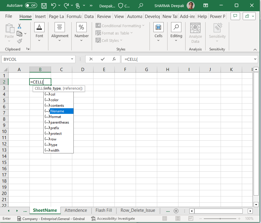
Type “=CELL” & press TAB, select option “filename” & press TAB, close the bracket, press ENTER.

This will give you the whole address of the Sheet, including the file name, folder name etc.

But we need to take only the File name.

So, for this purpose I will use MID, FIND Functions along with CELL.

Refer to the below formula.

=MID(CELL("filename"),FIND("[",CELL("filename"))+1,FIND(".",CELL("filename"))-FIND("[",CELL("filename"))-1)

How to get Excel Sheet Name

 

Hi Learners, in this blog post I will share how you can get the Excel sheet name.

Select a cell.

 

Type “=CELL” & press TAB, select option “filename” & press TAB, close the bracket, press ENTER.

 

This will give you the whole address of the Sheet, including the file name, folder name etc.

But we need to take only the Sheet name.

So, for this purpose I will use MID, FIND Functions along with CELL.

Refer to the below formula.

=MID(CELL("filename"),FIND("]",CELL(("filename")))+1,30) [Max. Length of Sheet name = 30 Char]

 

 

Change the “SheetName” to “SheetName_1”. It should read the new sheet name.

How to use Flash fill in MS Excel?

 

How to use Flash fill?

Hello friends, in this blog I will teach you how you can use Flash fill option in MS Excel.

Friend it is a magical option/tool.

It follows the pattern and takes action as per this pattern.

In below example, I have a column having complete name; first and last name in single cell.

I want to set First name and Last name in separate cells.

In Column C ( First Name) I write the first name; Suresh and hit the enter button.

Now go to ‘Data >> Flash Fill’ & click over there or just press ‘Ctrl + E’ and it will put the First names in the respective Rows.

 

Now type Last Name in column D, ‘Sharma’ and press enter.

Press ‘Ctrl + E’ and like before all last names will be set in column D in respective Rows.

 

 

 

How to use SUMIFS function in MS Excel?

In mathematics or any calculation, addition is the basic function or calculation, but sometimes we need to add some data with multiple conditions or criteria.

To do the conditional addition in MS excel there is a method for this task and this is very easy as well.

So let’s start doing SUMIFS in MS Excel.

What is SUMIFS function: This function adds the cells specified by a given condition or criteria.

Difference in SUMIF and SUMIFS is you can apply more than one criteria.

  

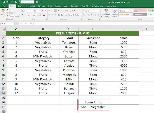
Open your MS excel file, put some data into it. For you, I have collected some data in the file as shown in below picture.

In first column (A) I have ‘S.No’, in second column (B) there is list of ‘Category’, in third (C); ‘Food’, fourth (D): ‘Salesman’ and in Fifth (E) there is ‘Sales’.

 

 

Here we want to find the sales done by the salespersons. If I want salesperson’s sale of Fruits and Vegetable separately then it should be calculated automatically.

In this example, I will calculate for Sonu’s sales for Fruits and Vegetables.

 

  Type ‘=SUMIFS’ in Cell E16 beside the Cell D16 (Sonu-Fruits), press the ‘tab’ key, function will be selected.

  

Now it is asking for

‘sum_range’, ‘criteria_range1’, and ‘criteria1’, and ‘criteria_range2’, and ‘criteria2’ so on.

sum_range: this is the range, which has to be summed, numerical value which are to be added.

I select the range from E3 to E14, since sales data is in column ‘E’.

criteria_range1 : select the range ( in column) with which you want to match the criteria1.

For example, in our case we want the total sales for category (Fruits & vegetables) by the salesmen, so we will select range from ‘Category’ (Column B).

Therefore, I select range from B3 to B14 and type ‘,’.

 

Now next is ‘criteria1’.

criteria1 : It refers to the first criteria for which SUM has to be done, this is the condition, in fact.

For this, I type “Fruits”. Since we want sales for Fruits only.

criteria_range2 : select the range ( in column) with which you want to match the criteria2.

For example, in our case we want the total sales by the salesmen, Sonu, so we will select range from ‘Salesman’ (Column D). So I select range from D3 to D14.

 

Now next is ‘criteria2’.

criteria2 : It refers to the second criteria for which SUM has to be done.

For this, I press ‘,’ then type “Sonu”, close the bracket and hit the ‘Enter’ key.

 

So, now we have the data of sales by Sonu, he sold Fruits of Rs. 1600 (800 + 800 = 1600).

Now I calculate the sales of Vegetables by Sonu.

Copy the formula; do not copy the cell, copy the text only and paste in cell E17 beside cell D17 (‘Sonu-Vegetable’) like below picture.

 

Change the “Fruits” into “Vegetables” and hit the ‘Enter’ key, it will sum the sales of Sonu for Vegetables.

  

You have the total sales of Sonu for vegetables only.

Sonu’s Total Sales for Vegetables = 1000 + 1000 = 2000.

 

So in the same manner you can make addition with various criteria or conditions.

So this all was about adding data for multiple specific criteria using SUMIFS function in MS Excel.

 

 

How to use SUMIF function in MS Excel?

In mathematics or any calculation, addition is the basic function or calculation, but sometimes we need to add some data with some condition. To do the conditional addition in MS excel there is a method for this task and these are very easy as well.

So let’s start doing SUMIF in MS Excel.

What is SUMIF function: This function adds the cells specified by a given condition or criteria.

Open your MS excel file, put some data into it. For you, I have collected some data in the file as shown in below picture.

In first column (A) I have ‘S.No’, in second column (B) there is list of ‘Category’, in third (C); ‘Food’, fourth (D): ‘Salesman’ and in Fifth (E) there is ‘Sales’.

Here we want to find the sales done by the salespersons. I want if I enter the name of the salesperson, total sales should be calculated automatically.

Like if I put Sonu in a cell then it should give me total sales by Sonu.

Like if I put Tinku in a cell then it should give me total sales by Tinku.

Type ‘SUMIF’, press the ‘tab’ key,  function will be selected.

Now it is asking for

range, criteria, and sum_range.

Range : select the range ( in column) with which you want to match the criteria.

For example, in our case we want the total sales for the salesmen, so we will select range from salesmen’s name.

So I select range from D3 to D14.

Now next is ‘criteria’.

Criteria : It refers to the criteria for which SUM has to be done.

For this, I press ‘,’ then select D16 cell reference, where I will put the name of salesman for which I want the total sales.

Now comes the ‘sum_range’.

Sum_range: this is the range, which has to be summed.

I select the range from E3 to E14, since sales data is in column ‘E’.

So total sales done by Sonu is 3200, you can verify it by adding Sonu’s sales separately.

Sonu: 1000 + 800 + 600 + 800 =  3200.

Now copy the formula, do not copy the cell, copy the test in the cell only and paste in Monu like below picture.

Change the Criteria from D16 to D17 and press ‘Enter’.

So total sales done by Monu is 4900, you can verify it by adding Monu’s sales separately.

Monu: 500 + 2000 + 400 + 2000 =  4900.

Now do the same procedure for Tinku.

Now copy the formula, do not copy the cell, copy the test in the cell only and paste in Tinku and change the Criteria from D17 to D18 and press ‘Enter’, like below picture.

So total sales done by Tinku is 6000, you can verify it by adding Tinku’s sales separately.

Tinku: 300 + 4000 + 500 + 1200 = 6000.

So this all was about adding data for a specific criteria using SUMIF function in MS Excel.

How to do SUM in MS Excel?

In mathematics or any calculation, addition is the basic function or calculation, to do the addition in MS excel there are two methods for this task and these are very easy as well.

So let’s start doing SUM in MS Excel.

Open your MS excel file, put some data into it. For you, I have collected some data in the file as shown in below picture.

In first column (A) I have ‘S.No’, in second column (B) there is list of ‘Item’, in third (C); ‘Qty’, fourth (D): Cost/Item and in Fifth (E) there is ‘Total Cost’.

To find total cost, I have multiplied Column C and D, as ‘=C2*D2’.

Now, we have to add all these Total Costs.

To do it, first type ‘=’ in Cell ‘E13’ and type ‘=E2+E3+E4+E5+E6+E7+E8+E9+E10+E11+E12’ and hit the ‘Enter’ key.

By doing this, we are adding all cells individually, but this method is useful when data is not in consecutive cells and small in quantity.

It means if we had to add data in cells E2, E5, E9, E12 then this method would very useful.

Since the data is in sequence and in consecutive manner then we do not need to use this method.

In MS we have a function called as SUM.

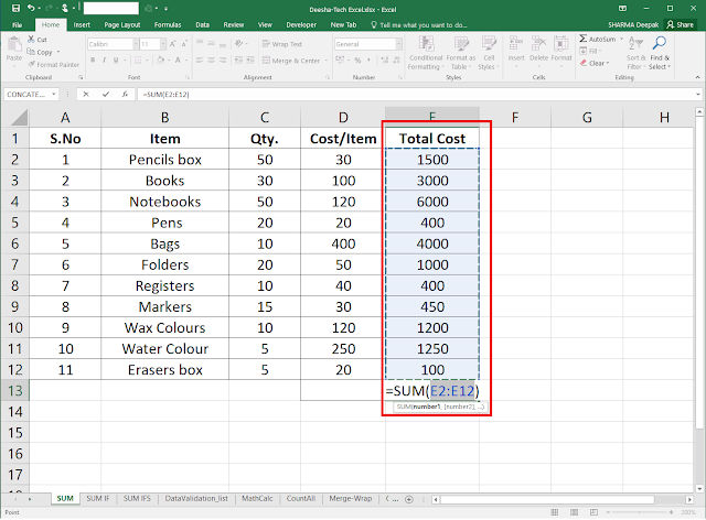
So to use this function, type ‘=SUM’ and it will look like the below picture.

Press ‘Tab’ key, SUM will be selected now it will ask for numbers, like number 1, [number 2].. and so on.

Now you can select the numbers individually as we did in previous example and you can also select a range, just click on the start cell and drag it to the desired cell.

I have selected start cell E2 and dragged to E12 then pressed the “Enter” Key, and we have the result; ‘=SUM(E2:E12)’ = 19300.

So, this was another method, but we have another method or a shortcut for this task.

That is ‘AutoSum’, this can be found in ‘Home’ tab under ‘Editing’ tools, as Home>Editing>AutoSum.

Select cell E13 and click on ‘AutoSum’ and it will automatically select all cells right above it, E2 to E12.

Keyboard Shortkey to this task is ‘ALT + =’.

So, this all was to add numbers in MS Excel.